Prediction of welfare outcomes for broiler chickens using Bayesian regression on continuous optical flow data
Published: May 29, 2014
By: Stephen J. Roberts (Department of Engineering Science, University of Oxford), Russell Cain and Marian Stamp Dawkins (Department of Zoology, University of Oxford)
J R Soc Interface. Dec 7, 2012; 9(77): 3436–3443. PMCID: PMC3481599
Published online Sep 5, 2012. doi: 10.1098/rsif.2012.0594
This journal is © 2012 The Royal Society
Published online Sep 5, 2012. doi: 10.1098/rsif.2012.0594
This journal is © 2012 The Royal Society
Abstract
Currently, assessment of broiler (meat) chicken welfare relies largely on labour-intensive or post-mortem measures of welfare. We here describe a method for continuously and robustly monitoring the welfare of living birds while husbandry changes are still possible. We detail the application of Bayesian modelling to motion data derived from the output of cameras placed in commercial broiler houses. We show that the forecasts produced by the model can be used to accurately assess certain key aspects of the future health and welfare of a flock. The difference between healthy flocks and less-healthy ones becomes predictable days or even weeks before clinical symptoms become apparent. Hockburn (damaged leg skin, usually only seen in birds of two weeks or older) can be well predicted in flocks of only 1–2 days of age, using this approach. Our model combines optical flow descriptors of bird motion with robust multivariate forecasting and provides a sparse, efficient model with sparsity-inducing priors to achieve maximum predictive power with the minimum number of key variables.
Keywords: animal welfare; optical flow; Bayesian multivariate modelling; variational Bayes inference
1. INTRODUCTION
Advance warning of undesirable outcomes such as outbreaks of disease, tail-biting in pigs, feather-pecking in hens and even rioting in human crowds would be a major step in controlling and even averting them altogether. In this context, changes in behaviour are increasingly being recognized as key precursors of such events with the possibility of indicating when and where husbandry changes would be most effective [1]. For example, even before overt clinical symptoms appear, a reduction in time spent at the feeder identifies those dairy cows that are most at risk of developing uterine inflammation after calving [2], a decline in exploration behaviour precedes and predicts clinical symptoms of disease in mice used as a model for Huntington’s disease [3], pigs that will later show a tendency to biting the tails of other pigs can be identified early by their tendency to bite other objects [4] and behavioural changes are shown by chickens with only sub-clinical levels of Salmonella [5]. At a group level, flocks of laying hens that subsequently go on to develop serious feather pecking by 40 weeks can be identified as early as 18–20 weeks, by increased incidence of disturbed behaviour [6].
Using behaviour in this way has a great advantage that it is non-invasive and does not require taking tissue samples for diagnosis. Furthermore, large numbers of animals can be monitored on a continuous basis, using easily available CCTV and video equipment. However, the potential of this approach has not yet been fully used because of a lack of ways of automatically analysing the vast quantities of behavioural data that can be produced. Unless behavioural precursors can be recognized automatically from camera data, their use as widely used diagnostics will be strictly limited.
Here, we show that statistical measures automatically derived fromsimple optical flow algorithms applied to the movements of large flocks of chickens can be combined to give highly predictive measures of health and welfare, some of them days or even weeks before more conventional measures are taken. The commercial broiler houses we recorded from each contained around 34 000 birds, all similar in appearance and with no possibility of marking or tagging individuals so that our methods could be applied to any situation where there is a need to monitor and analyse information about large numbers of anonymous individuals, such as crowds of people, or flocks and herds of animals. The use of optical flow to analyse behaviour at a group level avoids the heavy computation involved in attempting to track many individuals at once. The computation required by our method is simple enough to be done in real time, giving a continuous minute-by-minute output.
Three basic statistical measures of optical flow (daily mean, skew and kurtosis) have already been shown to be predictive on their own of key health and welfare measures in broiler chickens [6,7]. Skew and kurtosis, as measures of heterogeneity of flow, were particularly effective at predicting final flock mortality, incidence of hockburn (damaged leg skin) and poor walking in older birds (27–35 days) even when the birds were as young as 15–20 days. In this study, we show the predictive power of this approach by using the optical flow measures as input to a Bayesian multivariate linear regression model, with sparsity-inducing shrinkage to highlight which variables are genuinely contributing to the predictive power of the model. Variables that contribute little information are then associated with very small factor weights, while those that contribute a great deal are weighted heavily. The result is a sparse, efficient model that gives the maximum predictive power with the minimum number of key variables.
By using information from different inputs and cumulating this information over the entire preceding life-history of a flock, we show that it is possible to predict end-of-flock welfare measures in birds as young as a week old and over a month before these measures are conventionally taken. The regression model described has potential application to a wide variety of other situations with multiple inputs and high levels of noise.
2. METHODS
2.1. Animals and housing
Data (optical flow, production and welfare) were collected from 24 commercial chicken flocks, all on a single site in the UK and belonging to a major producer company. Four flocks were studied at a time, housed in separate identical broiler houses, each with floor area of 1670 m2 and with identical numbers and layout of feeders, drinkers and ventilation fans. The same farm staff looked after all the flocks. Six replicates of four flocks were completed over the period between October 2010 and June 2011. Each flock contained approximately 34 000 chickens of mixed sexes and two commercial broiler breeds (sometimes separated and sometimes mixed, according to company needs). Chicks were placed as day-olds and grown to 35 days old with a target final stocking density of 38 kg m-2. Flocks were not thinned (proportion of flock removed before clearance) during the growing period.
2.2. Production and welfare data
The company provided the following data for each flock: % mortality (% of all deaths before slaughter), % culls (% of all birds killed before slaughter because of leg problems), daily mortality, daily culls, daily weights (manually weighed), daily growth rate, daily water consumption, daily food consumption, % pododermatitis (% birds scored with foot pad lesions after slaughter at the slaughter plant) and % hockburn (% of birds scored with problematic ‘brown hocks’ after slaughter at the slaughter plant). To assess the walking ability of living birds, a trained observer used the six-point Bristol Gait Score [8] with a catching pen and gait scored 60 (randomly selected) birds on day 28. The measurements were monitored by independent measurements from a second observer. The results were expressed as the mean gait score for that flock. The observers used a catching pen placed at the same positions in each house. The 24 flocks showed a mean mortality of 3.35 per cent (s.d. = 0.91; range 2.37–6.46%) and an average gait score of 1.92 (s.d. = 0.23; range 1.64–2.38). We note, particularly, the very narrow range of both mortality and gait scores, indicating that these data are well suited to testing the sensitivity of our methods.
2.3. Cameras and hardware
Optical flow was monitored continuously between 08.00 and 20.00 h, using a bespoke recording processing unit1 designed to operate continuously in the demanding conditions of commercial broiler houses and with enough capacity to store 90 days of data. The lights were continuous during the recordings.
2.4. Optical flow analysis
Most automated visual-processing techniques keep track of individual animals, which is a very difficult task especially with large numbers of animals unless they are marked and even then is computationally prohibitive. Instead, we extract motion from the chickens as a whole group, using an optical flow algorithm. This was facilitated by the fact that broiler chickens are white, in contrast to their darker background. An optical flow is an approximation to apparent velocities of image motion and can be used to describe the mass movement of a group of objects. We use here the Lucas–Kanade optical flow method [9,10], in which incremental motion in the stack of images, f(x,y,t,), is estimated as follows.
Let f(x,y,t) be the grey-level at pixel x,y at time t. Consider the expansion of partial derivatives
if f remains a constant function (brightness), then df ≈ 0 whence
where v ≈ def (vx ; vy)T is the velocity vector. The most commonly used method to estimate velocities is the Lucas–Kanade method which places a small neighbourhood around the pixel of interest, in which it is assumed that the motion vector is stationary. If we define the set fp1; p2; . . . ; png as the pixels in the neighbourhood, then
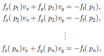
which can be written in the form
Av = b;
Figure 1. Correlations, r, of day-by-day regression onto (a) final mortality, (b) hockburn and (c) expert gait score. The solid horizontal lines represent the p = 0.05, p = 0.01 boundaries and each subplot shows the data (dots) along with best-fit regression (solid thick curve) and associated ±1; 2 standard posterior uncertainty (thin curves, dashed curves respectively).

with solution given as
i.e. using the pseudo inverse of A. The matrix A here is the matrix of spatial partial derivatives over the set of pixels in a neighbourhood, and b is the column vector of (negative) partial derivatives with time

The optical flow algorithm was executed in situ by the Fit-2 computer inside each Black Box unit, using 15 min blocks of recorded video footage from each camera and alternating between its two cameras. Consider a video file that consists of T image frames each of 320 x 240 pixels. Each image is divided into 1200 (=40 x 30) eight-by-eight pixel blocks. The optical flow algorithm estimates, for each block, a local velocity vector derived by analysis of the frame-by-frame changes between two consecutive image frames at time t and t + 1. The velocity vector contains two elements, horizontal and vertical, i.e. v[t; l] = (vx [t;l]; vy[t;l]T, for frames at time t = 1; . . . ;T, and blocks l = 1; . . . ; 1200. From the velocity vectors, the amount of movement for each block was obtained as the magnitude of the velocity, V[t;l] = |v|. As a snapshot of global movement statistics at time t, the spatial mean, variance, skewness and kurtosis of V[t;l] were sequentially calculated for each frame in the video file, resulting in a multivariate (four-dimensional) timeseries of length t = l . . .T samples. Each camera recorded data in a series of 15 min blocks throughout the day, and in the analysis presented in this study, we average over all daily blocks to obtain an aggregate measure of daily mean flow, variance, skewness and kurtosis, giving rise to a daily four-dimensional vector characterizing the birds’ motion.
3. RESULTS
The dataset was analysed using a Bayesian multivariate linear model with shrinkage, such that sparsity-inducing priors are placed over the factor weights in the model, leading to weights associated with inputs that have little information regarding the target regression to shrink towards zero. There are two main reasons for this choice. Firstly, given a relatively small, independent dataset size (remember that the number of trials is 24), we should naturally bias our analysis towards simpler models, thus mitigating against potentially poor generalization due to overfitting. Secondly, we may entertain a simple, yet effective, shrinkage mechanism that we can relate directly to factor weights associated with the optical flow parameters over time. The mathematical details of the approach are given in full in the appendix of this study, with particular details of the inputs to the model being covered in the final subsection. All the results we present in the data are strictly causal; i.e. we regress onto future values of welfare and include in our models only observations from the past.
The model predictions based on combined (mean, variance, skew and kurtosis) optical flow daily aggregate measures for individual days are shown in figure 1. Figure 1a shows that the model predicts total flock % mortality when the chickens are only 15 days old. Figure 1b shows similar predictions for hockburn, 20 days or so before hockburn is assessed (at the slaughterhouse). The predictions for gait score become significant by day 13, even though gait scoring was not carried out until day 28. The solid horizontal lines represent the p = 0.05, p = 0.01 boundaries, and each subplot shows the data (dots) along with best-fit regression (solid thick curve) and associated ±1; 2 standard posterior uncertainty (thin curves and dashed curves, respectively). The latter is not used in any of our analysis and is offered solely to highlight the underlying trend. This regression was performed using a Bayesian model with spline basis functions, based upon the model presented in the appendix. Details of the approach may be found in the final subsection of the appendix. Figure 2 depicts the factor weights associated with this set of predictions, for each of the three welfare measures, broken down by optical flow statistic. We note that mean optical flow has dominantly negative factor weights in all cases, variance is not significantly related, and both optical flow skewness and kurtosis are positively related to the welfare measures. We note that increases in these measures are indicative of welfare problems and hence should be associated with lower optical mean flows, indicative of birds that are less able to move. A positive skewness is associated with a longer tail to the right and a leftdominant peak, again compatible with our hypothesis of populations of less-able moving birds. The positive factor weighting of kurtosis indicates a potential population spread with the emergence of a low-mobility group of birds.
Figure 2. Boxplots of optical flow factor weights aggregated from the predictions shown in figure 1 for (a) final mortality, (b) hockburn and (c) expert gait score.

Figure 3. Correlations, r, of running regression onto (a) final mortality, (b) hockburn and (c) expert gait score. The solid horizontal lines represent the p = 0.05, p = 0.01 boundaries, and each subplot shows the data (dots) along with best-fit regression (solid thick curve) and associated ±1; 2 standard posterior uncertainty (thin curves and dashed curves, respectively). We note the improved prediction performance of hockburn and gait score.

The previous model used optical flow observations from each day in turn to forecast welfare measures. Figure 3 shows the effect on the models predictions of including optical flow data not just from one day at a time (as in figure 1) but from a given day and all preceding days for that flock. The vector of information hence grows as we proceed on a day-by-day basis. We see that the predictions for mortality are not much changed (figure 3a), but both % hockburn and gait score are accurately predicted from a much earlier age. Particularly, we see that there is a very significant early correlation with final % hockburn (figure 3b) and with expert gait score (figure 3c).
4. DISCUSSION
These results clearly show the increased predictive power that can be obtained from combining individual optical flow measures into a single Bayesian regression model and using the cumulative information that can be obtained from data collected continuously over time. The narrow range of recorded mortalities and gait scores in the flocks used for this analysis showed that the method is sensitive enough to discriminate between similar flocks and therefore has potential as a commercial management tool. It appears to be particularly effective at predicting which flocks are at risk of hockburn or walking defects. This is particularly clear for predicting which flocks will develop high levels of hockburn and which ones will have significant numbers of birds with walking problems.
Hockburn is a form of contact dermatitis caused by birds sitting for long periods on wet, poor-quality litter [11,12]. Ammonia from faecal matter in the litter damages the skin and leaves black or brown lesions on the legs. It is used as a measure of welfare in its own right because, although usually assessed post mortem, it gives an indication of the conditions that have been experienced by a bird during its lifetime [11]. The first signs of hockburn may appear as early as two weeks of age [12] and an indication that a flock that will end up with a high % of hockburn in birds after slaughter include the weight and density of the birds at two weeks [13] and high skew and kurtosis of optical flow at the same age [7]. By predicting which flocks will have later hockburn problems from optical flow information in the first few days of life, the model thus seems to be able to give a warning at a very early stage, before overt symptoms appear. Simply using the amount of movement is not enough, because the mean level of optical flow is not, on its own, sufficient to predict later hockburn at least until 15 days [7]. It is only with the full predictive power of all the available optical flow measures that the model provides that flocks at risk of hockburn can be identified.
A similar increase in predictive power is shown by the model’s ability to predict gait score. The skew and kurtosis of optical flow, taken separately, allow prediction of which flocks are likely to be scored as having a high % of poor walkers over a week before the gait scoring is actually carried out, i.e. on day 18–20 when gait scoring is done on day 28 [7]. The model, however, allows such predictions to be made much earlier in the birds lives when they are only 5 or 6 days old—over three weeks before actual gait scoring was carried out. As young birds with severe walking difficulties would be culled well before 28 days (and would therefore not be present for the formal gait scoring), the model must be using information about the optical flow caused by the movement of the remaining birds that may be walking healthily in their first week but will, nevertheless, by the age of 28 days, be part of a flock that that has a significant number of birds with gait deficiencies.
The ability to predict health and welfare problems before they become serious is an important way in which producers can improve both the production and welfare of their animals through early diagnosis and husbandry changes, such as increasing house ventilation. The Bayesian model described here automatically extracts key information from the optical flow patterns made by flocks of broiler chickens. It is, however, equally suitable for a wide range of other applications wherever there is a need for ‘early warnings’ in continuous real-time data.
This work was partly funded via the UK BBSRC, to whom we are grateful. The authors thank Andy Morris for his generous help in collecting the data and Sibo (Spark) Lu for his help with developing the recording devices.
APPENDIX A. BAYESIAN MULTIVARIATE LINEAR MODEL WITH SHRINKAGE
We start by recasting the multivariate linear model discussed in this study such that the observed y(x) is modelled as a noise-corrupted linear combination of a set of B-dimensional observations, øi , which are indexed via an independent variable x (this represents an index into the data array, for example and equates to a timing index in our application).

in which wi are the factor weights, w0 a bias, or offset, term and øi(Χ) is the observable set indexed to variable x. The noise term, h, is taken to be drawn from a normal distribution, N(0;b-1), in which b is the precision (inverse variance). Without loss of generality, we may augment the observation set with a column of ones, and so fold w0 and [wi] into a single vector w and rewrite the above as
where ø is the (B + 1)-dimensional vector composed of all B observed variables associated with x and a column of ones.
A.1. Maximum likelihood
The maximum likelihood (ML) solution for the weights is given by the standard pseudo-inverse equation, namely
where Y is the array of all observed (y1; y2; . . . ; yN) associated with X = (x1; x2; . . . ; xN) and Ø is the matrix of all observables over all xi € X (and so is of size B x N). The problem with the ML approach, however, is model-overfitting. Some relief from the inherent problems associated with ML solutions may be obtained by introducing a prior over the weights and obtaining the maximum a posteriori solution. This approach still relies on point values and fails to take into account the intrinsic uncertainty by marginalizing over the posterior distributions of the variables, thus providing a full Bayesian solution. While the latter could be achieved using, for example, sample-based approaches. In the sampling framework, integration is performed via a stochastic sampling procedure such as Markov chain Monte Carlo. The latter, however, can be computationally intensive, scales poorly and assessment of convergence is often problematic. In this paper, we advocate an alternative solution based on the variational Bayes (VB) framework. In recent years, VB has been extensively used as a method of choice for approximate Bayesian inference as it offers computational tractability even on very large datasets. A full tutorial on VB is given in [14,15]. In what follows, we describe the key features and concentrate on the derivations of update equations for the linear basis model at the core of this study.
A.2. The probabilistic model
To start with, let us consider our Bayesian model such that the weights wi are all drawn from a zero-mean Gaussian distribution with an isotropic covariance having precision (inverse variance) α
As α ≥ 0; the precision hyperparameter has a gamma distribution with hyper-hyperparameters bα; cα:
The noise term, h, is taken as zero-mean with precision hyperparameter Β over which we place another Gamma distribution
We concatenate all the parameters and hyperparameters of the model into the vector Ø=[w,α,β]. As the weights depend on the scale α (but not on the noise precision β); the joint distribution over Ø factorizes as
APPENDIX B. VARIATIONAL BAYESIAN INFERENCE
The central quantity of interest in Bayesian learning is the posterior distribution p(Ø| data); which fully describes our knowledge regarding the parameters of the model, Ø. Given a probabilistic model of the data with parameters Ø; the ‘evidence’ or ‘marginal likelihood’ of the data under the model is given by
The log evidence can be written as

where q(Ø|D) is a tractable posterior proposal density. This has been introduced in both denominator and numerator in equation (B 2). Hence,

We may write the latter equation as
where
is known as the (negative) variational free energy and
is the Kullback–Leibler (KL) divergence between the approximate posterior q() and the true posterior p().
Equation (B 4) is the fundamental equation of the VBframework. Importantly, because the KL-divergence is always positive, F(p,q) provides a strict lower bound on the model evidence. Moreover, because the KL-divergence is zero when the two densities are the same, F(p,q) will become equal to the model evidence when the approximating posterior is equal to the true posterior, i.e. if q(Ø|D) = p(Ø|D).
The aim of VB-learning is therefore to maximize F(p,q) and so make the approximate posterior as close as possible to the true posterior. This requires the extremization of an integral with respect to a functional, which is typically achieved using the calculus of variations. However, to obtain a practical inference algorithm, we can ensure that extremization with respect to the function q(Ø) can be replaced exactly by extremization with respect to the parameters Ø. This holds so long as the distributions are in the exponential family.
As this includes all the commonly used probability distributions, this constraint is not normally problematic. What we obtain is then a set of coupled update equations over the parameters that are cycled until a convergence criterion is met. This approach is a generalization of the expectation–maximization (EM) algorithm, which is obtained as a special case of variational Bayes in the limit of the q() distributions being replaced by delta functions at their ML values [14].
We consider parameter Øi , and define f (Øi) as the marginal integral over all other Ø-i , where we use the nomenclature i to mean ‘all variables except for i’,
The update form can be shown to be such that the updated distribution for parameter Øi is
In the next subsections, we cycle through the parameters of the model, detailing the update equations associated with each q() distribution in turn. In the following sections, we use Ø to denote the ‘new’, updated variable and Ø0 to be the prior value (i.e. our initialization). We note that, such as the EM algorithm, each iteration is guaranteed to improve the marginal likelihood of the data under the model.
B.1. Updating the weight parameters, w
We begin by defining

Our update equations, which maximize the functional, are hence given via
Substituting for the terms in equation (B 9) gives
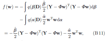
where α and Β are the mean weight and noise precisions from the posterior distributions over α and Β (see next two sections). The weight posterior is therefore a normal density q(w|D) = N (w; w; ε); where

where I denotes the identity matrix. Thus, the posterior precision matrix, ε-1, takes the usual Bayesian form of being the sum of the data precision, plus the prior precision, ^αI. With ^α = 0, i.e. no prior on the weights, we recover the ML solution of equation (A 3).
B.2. Updating the weight precision, a
We let

As before, the negative free energy is maximized when
By substituting for the terms in equation (B 13), we find that the updated weight precision posterior density is a gamma density of the form q(α|D) = ⊆(α; βα, Cα) where the updated hyper-hyperparameters, ^ba and ^ca; are given by
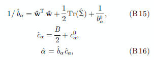 where B is the number of basis functions.
B.3. Updating the noise precision, b
Again, we start by writing the function

The negative free energy is then maximized when
By substituting for the terms in equation (B 17) we find, as with a, that the posterior distribution over β is of gamma form, q(β|D) = ς(β; bβ, cβ) with updates to the hyper-hyperparameters ^bβ and ^cβ given by
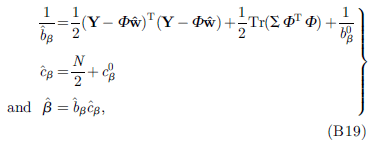
where N is the number of data points.
B.4. Structured priors
Instead of using the isotropic Gaussian of equation (A 4), where the distribution over all the weights has a common scale (defined by the single hyperparameter α), we can split the weights into groups and allow different groups to have different scales in their distributions; each weight wi can indeed have its own scale hyperparameter. This approach is often referred to as automatic relevance determination [14,16,17], so-called because by inspecting the inferred scales associated with the weights, we can see which (groups of ) weights are relevant to the problem at hand; those that are not helpful to our problem will evolve with distributions with vanishingly small variance, i.e. there is strong evidence that the weight lies close to zero. Conversely, those weights that are well supported by the data will entertain larger variances in their pdfs. The importance of this lies with each weight acting as a scaling associated with an observed variable (denoted here via the fi). Hence, weights that are unsupported by the data shrink to close to zero because their associated variable is not explanatory of the data. This means we may operate with a rich set of observed variables and allow the Bayesian model to select only those that have explanatory power in the data.
For our linear models, we want to allow for different wi to have such different scales, and this property can be captured with ‘structured priors’. For example, if we have strong domain knowledge that certain parameters should have a similar posterior scale, then we can group them. Our structured priors are hence of the form:

where the weights have been split into j = 1 . . .G groups with Bj weights in the jth group and where we define

with Ij being a matrix with 1s along the diagonal that pick off coefficients in the jth group, and zeros elsewhere. Use of structured priors results in VB updates for the posterior weight covariance and weight precision as follows:
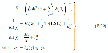
The other updates are exactly the same as for the global variance scale over the parameters.
B.5. Application details
The above methodology is used twice within this paper. Once for forecasting future welfare variables and secondly for fitting a trend curve to the results. The latter usage does not form part of the analysis, and the trend curve is solely used for making presentation of the data clearer. These two cases are detailed as follows.
Forecasts: In our forecasts, the target variables are welfare measures and the observations vector, Ø(x) are the optical flow statistics either observed on day x or from all days 1 to x. In the former case, Ø is a fourdimensional vector of optical flow mean, variance, skewness and kurtosis. In the latter case, Ø is a vector of increasing length, as it represents a vector of optical flow statistics from each day prior to and including day x.
Trend curves: To form smooth trend curves through the day-by-day correlations of our forecasts with the welfare targets, we exploit the above model with Ø being a set of thin-plate spline basis functions, one centred on each day of our results. The spline functions are given by
where xi are locations of the spline basis functions, here located at each day of the study.
REFERENCES
1 Koolhaas, J. M. 2008 Coping style and immunity in animals: making sense of individual variation. Brain Behav. Immun. 22, 662–667. (doi:10.1016/j.bbi.2007.11.006)
2 Urton, G., von Keyserlingk, M. A. G. & Weary, D. M. 2005 Feeding behavior identifies dairy cows at risk for metritis. J. Dairy Sci. 88, 2843–2849. (doi:10.3168/jds. S0022-0302(05)72965-9)
3 Littin, K., Acevedo, A., Browne, W., Edgar, J., Mendl, M., Owen, D.,Sherwin, C.,Wurbel, H.&Nicol,C. 2008Towards humane end points: behavioural changes precede clinical signs of disease in a Huntingtons disease model. Proc. R. Soc. B 275, 1865–1874. (doi:10.1098/rspb.2008.0388)
4 Beattie, V. E., Breuer, K., O’Connell, N. E., Sneddon, I. A., Mercer, J. T., Rance, K. A., Sutcliffe, M. E. M. & Edwards, S. A. 2005 Factors identifying pigs predisposed to tail biting. Anim. Sci. 80, 307–312. (doi:10.1079/ ASC40040307)
5 Toscano, M. J., Sait, L., Jorgensen, F., Nicol, C. J., Powers, C., Smith, A. L., Bailey, M. & Humphrey, T. J. 2010 Sub-clinical infection with salmonella in chickens differentially affects behaviour and welfare in three inbred strains. Br. Poult. Sci. 51, 703–713. (doi:10.1080/ 00071668.2010.528748)
6 Lee, H.-J., Roberts, S. J., Drake, K. A. & Dawkins, M. S. 2011 Prediction of feather damage in laying hens using optical flow and Markov models. J. R. Soc. Interface 8, 489–499. (doi:10.1098/rsif.2010.0268)
7 Dawkins, M. S., Lee, H.-J., Waitt, C. D. & Roberts, S. J. 2009 Optical flow patterns in broiler chicken flocks as automated measures of behaviour and gait. Appl. Anim. Behav. Sci. 119, 203–209. (doi:10.1016/j.applanim.2009.04.009)
8 Kestin, S. C., Knowles, T. G., Tinch, A. E. & Gregory, N. 1992 Prevalance of leg weakness in broiler chickens and its relationship with genotype. Vet. Rec. 131, 190–194. (doi:10.1136/vr.131.9.190)
9 Beauchemin, S. & Barron, J. 1995 The computation of optical flow. ACM Comput. Surv. 27, 433–467. (doi:10. 1145/212094.212141)
10 Fleet, D. J. & Weiss, Y. 2005 Optical flow estimation. In Handbook of mathematical models for computer vision (eds N. Paragios, Y. Chen & O. Faugeras), pp. 239–258. New York, NY: Springer.
11 Haslam, S. M., Brown, S. N., Wilkins, L. J., Kestin, S. C., Warriss, P. D. & Nicol, C. J. 2006 Preliminary study to examine the possibility of using foot burn or hockburn to assess aspects of housing conditions in broiler chickens. Br. Poult. Sci. 47, 13–18. (doi:10.1080/00071660500475046)
12 Kjaer, J. B., Su, G., Nielsen, B. L. & Sa¨renson, P. 2006 Foot pad dermatitis and hock burn in broiler chickens and degree of inheritance. Poult. Sci. 85, 1342–1348.
13 Hepworth, P. J., Nefedov, A. V., Muchnik, I. B. & Morgan, K. L. 2010 Early warning indicators for hock burn in broiler flocks. Avian Pathol. 39, 405–409. (doi:10.1080/03079457.2010.510500)
14 Bishop, C. M. 2006 Pattern recognition and machine learning. New York, NY: Springer.
15 Fox, C. W. & Roberts, S. J. 2012 A tutorial on variational Bayesian inference. Artif. Intell. Rev. 38, 1–11. (doi:10. 1007/s10462-011-9236-8)
16 Neal, R. 1998 Assessing relevance determination methods using DELVE. In Neural networks and machine learning (ed. C. Bishop), pp. 97–129. Berlin, Germany: Springer-Verlag.
17 Penny, W. & Roberts, S. 2002 Bayesian multivariate autoregressive models with structured priors. IEE Proc. Vision, Image Signal Proc. 149, 33–41. (doi:10.1049/ ip-vis:20020149)
Related topics
Authors:
Join to be able to comment.
Once you join Engormix, you will be able to participate in all content and forums.
* Required information
Would you like to discuss another topic? Create a new post to engage with experts in the community.
Create a post4 de junio de 2014
Dear Professor Marian Dawkins,
This is a great effort to predict problems early during close house broiler rearing with high inputs. With a an input density of about 23.4 birds per squire meter, I have observed about 20% skin damages. One of the factors observed for this is the noise of automatic feeders at the start. Didn't you consider this factor as one of the welfare related?
D.C. Hettiarachchi






.jpg&w=3840&q=75)